Gravitational Acceleration
Every body in the system attracts every other body according to Newton’s Law of Universal Gravitation. For body , the net acceleration due to all other bodies is:
where is the distance between the two bodies and is the unit vector pointing from toward .
Why Initial Velocity Matters
Gravity alone will pull every body straight toward every other body. What prevents them from colliding is their initial velocity — the sideways motion that turns a free-fall into a curved orbit. This is the same reason the Moon doesn’t crash into the Earth: it’s falling toward us constantly, but it’s also moving sideways fast enough that it keeps missing.
When you call add_body(), the vx,
vy, vz parameters set this initial velocity.
The balance between speed and distance determines the shape of the
orbit. At a given distance
from a central mass
,
the circular orbit velocity is:
If the body’s speed exactly matches this, it traces a perfect circle. Faster and the orbit stretches into an ellipse (or escapes entirely if ). Slower and the orbit drops into a tighter ellipse that dips closer to the central body. With zero velocity, the body falls straight in — no orbit at all.
Gravitational Softening
When two bodies pass very close,
and the acceleration diverges toward infinity. This is a well-known
numerical problem in N-body codes. orbitr offers an
optional softening length
that regularizes the potential:
With softening enabled, close encounters produce large but finite
forces instead of blowing up to NaN. Set
softening = 0 (the default) for exact Newtonian gravity, or
try something like softening = 1e4 (10 km) for dense
systems.
Numerical Integration Methods
simulate_system() offers three methods for stepping the
system forward through time. All operate in 3D Cartesian
coordinates.
1. Velocity Verlet (default, method = "verlet")
A second-order symplectic integrator. It conserves energy over long timescales, making it the gold standard for orbital mechanics. Orbits stay closed and stable indefinitely.
The position is advanced first, then the acceleration is recalculated at the new position, and finally the velocity is updated using the average of the old and new accelerations. This requires two acceleration evaluations per step (the main cost), but the payoff in stability is enormous.
2. Euler-Cromer (method = "euler_cromer")
A first-order symplectic method. It updates velocity first, then uses the new velocity to update position. This small reordering prevents the systematic energy drift that plagues standard Euler:
Faster than Verlet (one acceleration evaluation per step) but less accurate. Good for quick previews.
3. Standard Euler (method = "euler")
The classical textbook method. Position and velocity are both updated using values from the current time step:
This artificially pumps energy into the system, causing orbits to spiral outward over time. Included primarily for educational comparison — use Verlet for real work.
Comparing the Three Methods
library(orbitr)
library(dplyr)
#>
#> Attaching package: 'dplyr'
#> The following objects are masked from 'package:stats':
#>
#>     filter, lag
#> The following objects are masked from 'package:base':
#>
#>     intersect, setdiff, setequal, union

system <- create_system() |>
  add_body("Star", mass = 1e30) |>
  add_body("Planet", mass = 1e24, x = 1e11, vy = 30000)

verlet <- simulate_system(system, time_step = 3600, duration = 86400 * 365, method = "verlet") |>
  mutate(method = "Velocity Verlet")

euler_cromer <- simulate_system(system, time_step = 3600, duration = 86400 * 365, method = "euler_cromer") |>
  mutate(method = "Euler-Cromer")

euler <- simulate_system(system, time_step = 3600, duration = 86400 * 365, method = "euler") |>
  mutate(method = "Standard Euler")

bind_rows(verlet, euler_cromer, euler) |>
  filter(id == "Planet") |>
  ggplot2::ggplot(ggplot2::aes(x = x, y = y, color = method)) +
  ggplot2::geom_path(alpha = 0.7) +
  ggplot2::coord_equal() +
  ggplot2::theme_minimal()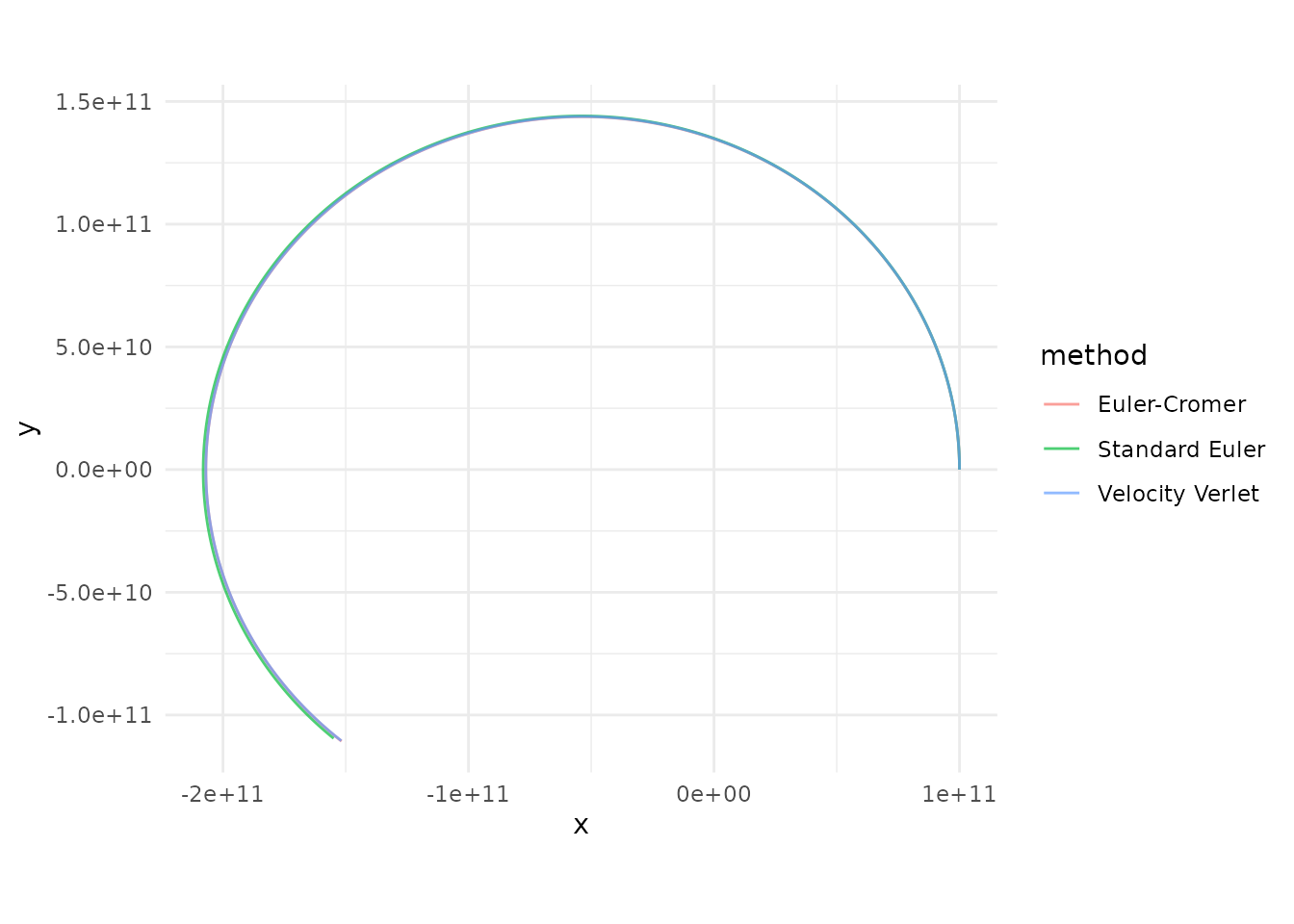
Verlet traces a clean closed ellipse, Euler-Cromer stays close but drifts slightly, and standard Euler spirals outward as it pumps energy into the orbit.
The C++ Engine
The inner acceleration loop is the computational bottleneck of any
N-body simulation. orbitr ships a compiled C++ kernel (via
Rcpp) that computes the
pairwise interactions in a tight nested loop. When the package is
installed from source with a working C++ toolchain,
simulate_system() automatically dispatches to this engine.
If the compiled code isn’t available, it falls back to a vectorized R
implementation that uses matrix outer products — still fast, but the C++
path is significantly faster for systems with many bodies.
You can control this with the use_cpp argument:
# Force the pure-R engine (useful for debugging or benchmarking)
simulate_system(system, use_cpp = FALSE)