Quick Start Guide • orbitr

Installation

# install.packages("devtools")
devtools::install_github("daverosenman/orbitr")

For 3D interactive plotting, you’ll also want:

install.packages("plotly")

Your First Simulation in 30 Seconds

orbitr is designed around a simple pipe-friendly workflow: create a system, add bodies, simulate, and plot.

library(orbitr)

create_system() |>
  add_body("Earth", mass = mass_earth) |>
  add_body("Moon",  mass = mass_moon, x = distance_earth_moon, vy = speed_moon) |>
  simulate_system(time_step = 3600, duration = 86400 * 28) |>
  plot_orbits()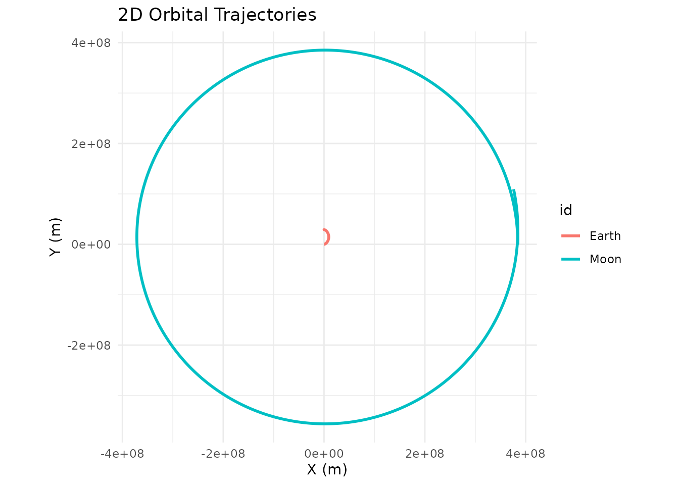

That’s it — a 28-day lunar orbit in four lines. Here’s what each step does:

create_system() initializes an empty simulation with standard gravitational constant G.
add_body() places a body with a given mass, position, and velocity. All positions are in meters, velocities in m/s. The built-in constants (mass_earth, distance_earth_moon, etc.) save you from looking anything up.
simulate_system() runs the N-body integration forward in time. time_step is how many seconds per integration step, duration is the total time to simulate.
plot_orbits() produces a quick 2D trajectory plot using ggplot2.

Customizing the Plot

By default, plot_orbits() returns a standard ggplot object for planar (2D) simulations and a plotly HTML widget for simulations with any 3D motion. (You can also force 3D rendering on planar data with three_d = TRUE.) Because the 2D case returns a regular ggplot, you can layer additional geoms, scales, themes, and labels onto it with + like any other ggplot.

A common annoyance is that the central body in a two-body system can be invisible: plot_orbits() draws each body as a geom_path() of its trajectory, and a much more massive body barely moves so its path is too small to see. The Sun in a Sun-Earth simulation is the classic example — it’s there, but its loop around the barycenter is well inside the Sun itself. The simplest fix is to drop a marker at the origin:

sim <- create_system() |>
  add_body("Sun",   mass = mass_sun) |>
  add_body("Earth", mass = mass_earth, x = distance_earth_sun, vy = speed_earth) |>
  simulate_system(time_step = 86400, duration = 86400 * 365)

sim |>
  plot_orbits() +
  ggplot2::geom_point(
    data = data.frame(x = 0, y = 0),
    ggplot2::aes(x = x, y = y),
    color = "gold",
    size = 6
  ) +
  ggplot2::labs(title = "Earth-Sun Orbit")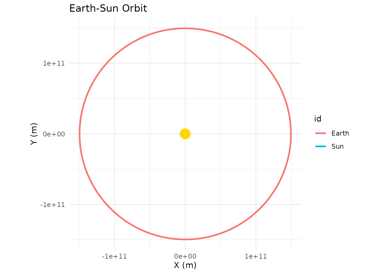

This works because the Sun sits essentially at the origin throughout the simulation. For systems where the central body actually moves a noticeable amount, you’d want to pull its position from the simulation tibble instead of hardcoding (0, 0).

Watching the Orbit in Motion

Static plots are nice, but you can also play the simulation forward as an animation with animate_system(). By default each body leaves a fading wake of recent positions behind it:

animate_system(sim, fps = 15, duration = 5)

animate_system() is the animated counterpart to plot_system() — it samples the simulation tibble down to roughly fps * duration evenly spaced frames, then renders them as a GIF using gganimate. Like the static plotters, it auto-dispatches to a 3D version (animate_system_3d(), an interactive plotly widget with a play button) the moment any body has non-zero Z motion. The 2D path requires the gganimate and gifski packages — install them with install.packages(c("gganimate", "gifski")).

Adding More Bodies

Since orbitr is a full N-body engine, you can add as many bodies as you want. Each one gravitationally interacts with every other. Here’s the Sun-Earth-Moon system for a full year:

create_system() |>
  add_body("Sun",   mass = mass_sun) |>
  add_body("Earth", mass = mass_earth, x = distance_earth_sun, vy = speed_earth) |>
  add_body("Moon",  mass = mass_moon,
           x = distance_earth_sun + distance_earth_moon,
           vy = speed_earth + speed_moon) |>
  simulate_system(time_step = 3600, duration = 86400 * 365) |>
  shift_reference_frame("Earth") |>
  plot_orbits()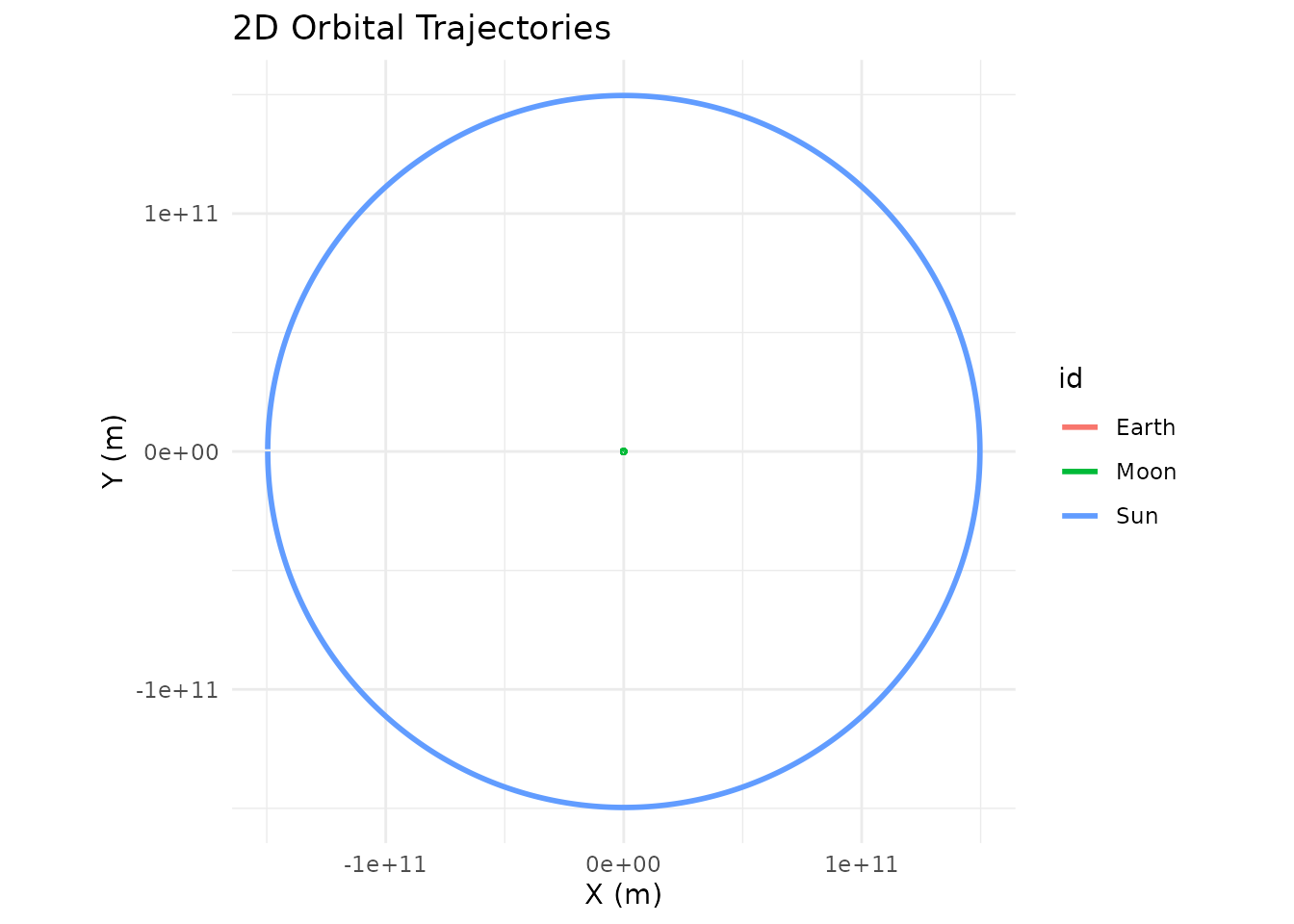

Notice shift_reference_frame("Earth") — this re-centers everything on Earth so you can see the Moon’s orbit instead of having everything overlap at the Sun’s scale.

Changing the Integrator

The default integrator is Velocity Verlet, which conserves energy and keeps orbits stable. You can switch to "euler_cromer" for faster (but less accurate) runs, or "euler" to see what happens when energy isn’t conserved:

create_system() |>
  add_body("Star", mass = 1e30) |>
  add_body("Planet", mass = 1e24, x = 1e11, vy = 30000) |>
  simulate_system(time_step = 3600, duration = 86400 * 365, method = "euler") |>
  plot_orbits()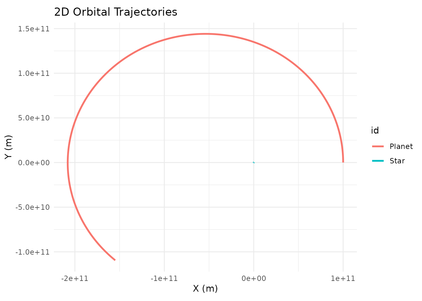

You’ll see the orbit spiral outward — that’s the Euler method artificially pumping energy into the system. Switch back to method = "verlet" for a clean closed ellipse.

The Output is Just a Tibble

simulate_system() returns a standard tidy tibble. You can use dplyr, ggplot2, plotly, or any other tool on it:

sim <- create_system() |>
  add_body("Earth", mass = mass_earth) |>
  add_body("Moon",  mass = mass_moon, x = distance_earth_moon, vy = speed_moon) |>
  simulate_system(time_step = 3600, duration = 86400 * 28)

sim
#> # A tibble: 1,346 × 9
#>    id       mass          x           y     z      vx          vy    vz  time
#>    <chr>   <dbl>      <dbl>       <dbl> <dbl>   <dbl>       <dbl> <dbl> <dbl>
#>  1 Earth 5.97e24         0         0        0   0        0            0     0
#>  2 Moon  7.34e22 384400000         0        0   0     1022            0     0
#>  3 Earth 5.97e24       215.        0        0   0.119    0.000571     0  3600
#>  4 Moon  7.34e22 384382520.  3679200        0  -9.71  1022.           0  3600
#>  5 Earth 5.97e24       860.        4.11     0   0.239    0.00229      0  7200
#>  6 Moon  7.34e22 384330083.  7358065.       0 -19.4   1022.           0  7200
#>  7 Earth 5.97e24      1934.       16.5      0   0.358    0.00514      0 10800
#>  8 Moon  7.34e22 384242692. 11036262.       0 -29.1   1022.           0 10800
#>  9 Earth 5.97e24      3438.       41.1      0   0.477    0.00914      0 14400
#> 10 Moon  7.34e22 384120357. 14713454.       0 -38.8   1021.           0 14400
#> # ℹ 1,336 more rows

Each row is one body at one point in time, with columns for position (x, y, z), velocity (vx, vy, vz), mass, body ID, and time.

Next Steps

The Physics — Understand the math behind the simulation
Examples — More complex systems including binary stars and the Kepler-16 system
Unstable Orbits — Why most random configurations are chaotic
3D Plotting — Interactive 3D visualization with plotly
Custom Visualization — Build your own plots with ggplot2 and plotly
Physical Constants — All built-in masses, distances, and speeds
Roadmap — Features being considered for future versions, plus a place to suggest your own